Bousssinesq's problem
Introduction
In Geomechanics, the Boussinesq's problem refers to the point load acting on a surface of an elastic half-space problem. The boundary conditions for this problem are:
- The load P is applied only in one point, in the origin.
- The load is zero in any other point.
- For any point infinitely distant from the origin, the displacements must all vanish.

Analytical solution
The analytical solution of the vertical displacement field is:
\[ u_z(x,y,z) = \frac{P}{4 \pi G d} (2 (1-\nu) + z^2 / d^2) \]
where \( G = \frac{E}{2(1+\nu)} \) is the Shear modulus of the elastic material, \( \nu \) is the Poisson ratio and \( d = \sqrt{ x^2 + y^2 + z^2 } \) is the total distance from load to the point.
MPM model and result comparison
For model the displacement field generated due the point load we will create an elastic body with dimensions \( l_x = l_y = l_z = 1 m \), for this we can use the keyword "cuboid", with point 1 in (0,0,0) and Point 2 in (1,1,1). For the elastic parameters of the material, we will use Young's modulus equal to \( E = 200e6 \) Pa, a density equal to \( \rho = 1500 kg/m^3\). This body is placed in a computational mesh with cell dimension \( dx = dy = dz = 0.1\) m. The boundary condition of this problem is a nodal load at the middle point on the body surface acting in vertical direction with magnitude of 1. For set this condition we will use the "nodal_point_load" keyword. The displacement boundary condition of the mesh is set using the "boundary_conditions" keyword. In this problem the plane Zn (upper plane) is set as free no move, and all the others planes are set as sliding, allowing movements only in parallel direction of the plane. The current MPM formulation solves the motion equation so, we need to add some damping to avoid the transient solution using "damping" keyword, with "kinetic" option for the damping's type. The "kinetic" keyword is used to active dynamic relaxations techniques on the velocity field for obtaining the static solution of the problem.
The input file for this problem is:
{
    "body":
    {
        "elastic-cuboid-body":
        {
            "type":"cuboid",
            "id":1,
            "point_p1":[0.0,0.0,0],
            "point_p2":[1,1,1],
            "material_id":1
        }
    },

    "materials":
    {
        "material-1":
        {
            "type":"elastic",
            "id":1,
            "young":200e6,
            "density":1500,
            "poisson":0.25
        }
    },

    "mesh":
    {
        "cells_dimension":[0.1,0.1,0.1],
        "cells_number":[10,10,10],
        "origin":[0.0,0.0,0.0],
        "boundary_conditions":
        {
            "plane_X0":"sliding",
            "plane_Y0":"sliding",
            "plane_Z0":"sliding",
            "plane_Xn":"sliding",
            "plane_Yn":"sliding",
            "plane_Zn":"free"
        }
    },
    "time":0.025,
    "time_step_multiplier":0.3,
    "results":
    {
        "print":50,
        "fields":["all"]
    },
    "nodal_point_load": [ [[0.5, 0.5, 1.0], [0.0, 0.0, -1.0]]],
    "damping":
    {
        "type":"kinetic"
    }
}
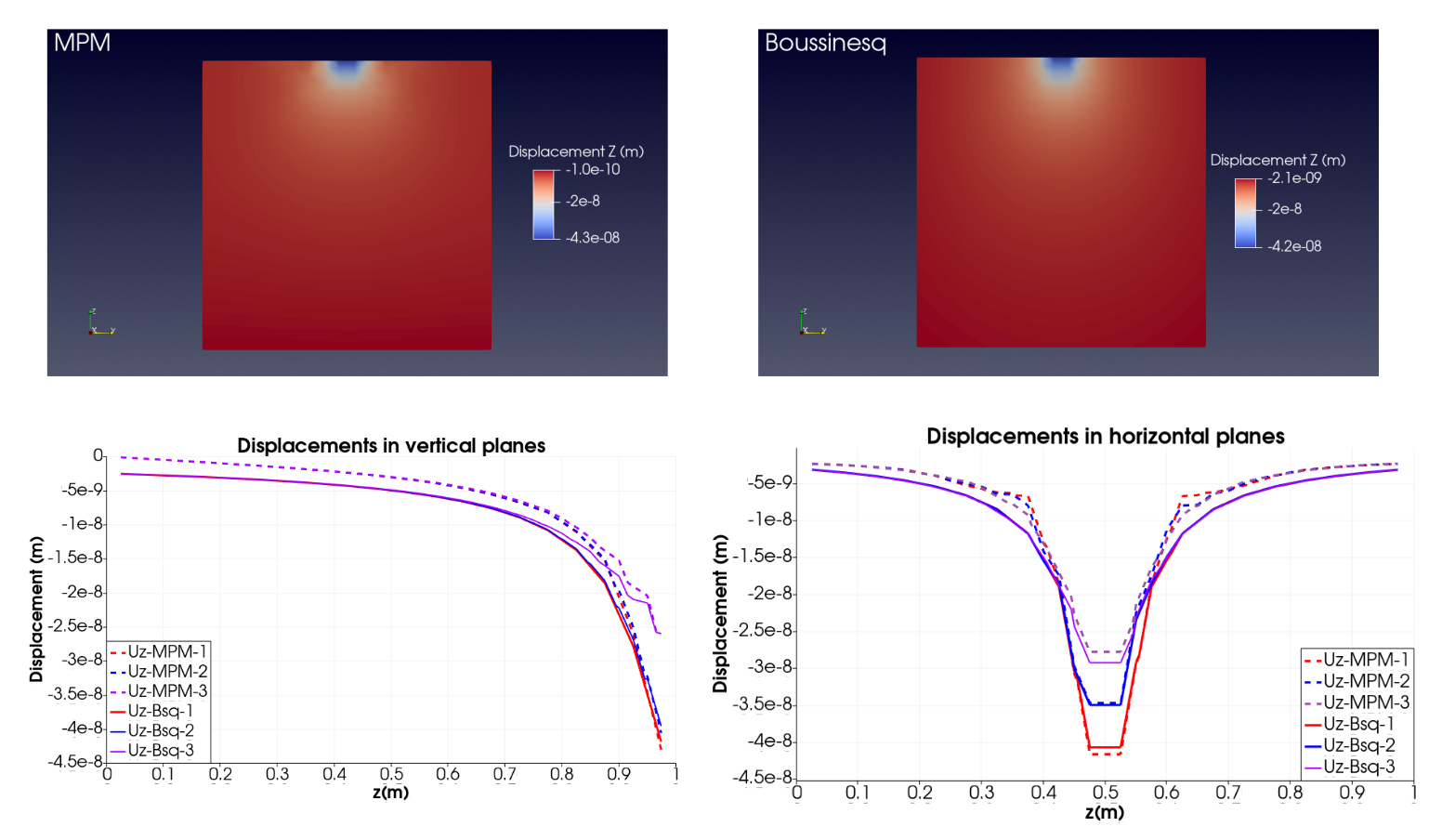
The numerical results obtained with MPM were compared with the analytical solution. In general the numerical solution presents a good coincidence with the analytical solution, however, some diferences are observed due the discretization. The MPM formulation uses particles to represent the continuum's variables in a Lagrangian approach. This particles represents a portion of the domain, so they have an associated volume. The particles do not represent a particle located at the boundary of the body and some errors, in consequence some differences will be observed. This differences must to be reducing with the refinement of the computational mesh.
Base acceleration example
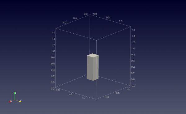
In this example we will show how to model the movement of an elastic body subjected to a dynamic boundary condition. The geometry of the body will be a regular cuboid with edge dimension \( l_x = 0.3\) m, \( l_y = 0.3 \) m, and \( l_z = 0.8 \) m in the \( xyz \) coordinate system. The lower coordinate point is located at \( p_{min} = (0.4, 0.4, 0.0) \) m. The dynamic boundary condition considered is a base acceleration defined as a function of time as \( \ddot{u} = A 2 \pi f cos ( 2 \pi f t + \alpha ) \). The total time of the simulation is 2 seconds, and the time step is \( \Delta t = 1e-4\) seconds. The material density considered is \( \rho = 2500 \) kg/m \(^3\), and the elastic behavior is defined by Young's modulus \( E = 100e6 \) MPa and Poisson ratio equal to \( \nu = 0.25 \). The figure below shows the body in the space.
MPM-Model
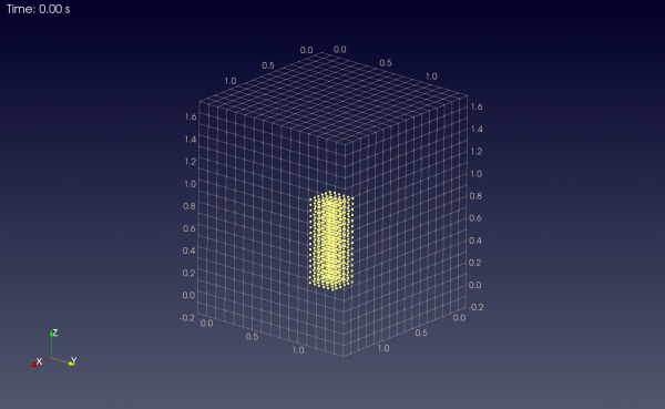
With these data we will to create an MPM model consisting in uniformly distributed particles inside the geometry of the body. For do so, we used the "body" and "cuboid" keywords. When body type is "cuboid" we can create a body with the lower and highest coordinate point P1 (lower) and P2 (hight) of the geometry. The material established using the "material_id" keyword. This material must to be correctly defined using the keyword "materials". When we create a body using uniformly distributed particles, eight in the case of a regular element mesh, the number of total particles in the body depends of the mesh grid cell dimension. In this case we will consider a uniform mesh consisting in elements of dimension \( \Delta x = \Delta y = \Delta z = 0.1 \) m. In a MPM model the mesh must to cover the whole domain, covering the complete amplitude of the body movement. For this example we will consider the same number of element in each direction \( n_x=12, n_y=12, n_z=15 \) to account from the origin of coordinate \( (0,0,0) \).
The complete JSON file with the keywords we write:
{ "stress_scheme_update":"USL",
"shape_function":"GIMP",
"time":10,
"time_step":0.0005,
"gravity":[0.0,0.0,0.0],
"n_threads":1,
"damping": { "type":"local", "value":0.0 },
"results": { "print":100, "fields":["id","displacement","velocity","material","active","body"] },
"n_phases":1,
"mesh": { "cells_dimension":[0.1,0.1,0.1], "cells_number":[10,10,15], "origin":[0,0,0]
},
"earthquake": { "active": true, "file": "base_acceleration.csv", "header": true } , "material": { "elastic_1": { "type":"elastic", "id":1, "young":10e6, "density":2500, "poisson":0.25 } },
"body": { "columns_1": { "type":"cuboid", "id":1, "point_p1":[0.2,0.2,0], "point_p2":[0.5,0.5,1.0], "material_id":1 }
} }
The "earthquake" block in the JSON input defines the parameters to activate seismic loading in the simulation and to specify the file containing the seismic record:
```json "earthquake": { "active": true, "file": "base_acceleration.csv", "header": true }
Where,
- active: Enables (true) or disables (false) the use of the seismic record.
- file: Path to the CSV file containing the seismic acceleration time series. The file must include at least four comma-separated columns: time, acceleration in X, Y, and Z directions.
- header: Indicates whether the CSV file includes a header row (usually true).
The record must to be the data in the following structure: time, acceleration_x, acceleration_y, acceleration_z. The five first lines of the acceleration record is:
t,ax,ay,az
0.0,-1.8849555921538759,-0.9424777960769379,-0.0
5e-05,-1.8849554991350466,-0.9424777844495842,-0.0
0.0001,-1.884955220078568,-0.9424777495675233,-0.0
0.00015000000000000001,-1.8849547549844674,-0.9424776914307561,-0.0
...
Once we have the JSON input file, we can execute the simulator with the input file as parameter. When the simulation ends we can find the particle results in the "/particle" directory, and the grid mesh in the "/grid" directory. The particles results are written in uniformly separated times determined by the number of results defined in the "print" keyword. The number of total results must be 40. In this example, the particles results must be "particle_1.vtu", "particle_2.vtu", ..., "particle_41.vtu". Together with the "particle_i.vtu" results, a particle serie file "particleTimeSerie.pvd" is created. This time series file can be used to load all the results in the Paraview scientific visualization program.
In other to visualize the results, the "particleTimeSerie.pvd" can be open in the Paraview by "> File > Open > particleTimeSerie.pvd". And the mesh can be loaded by open the "> File > Open > eulerianGrid.vtu".
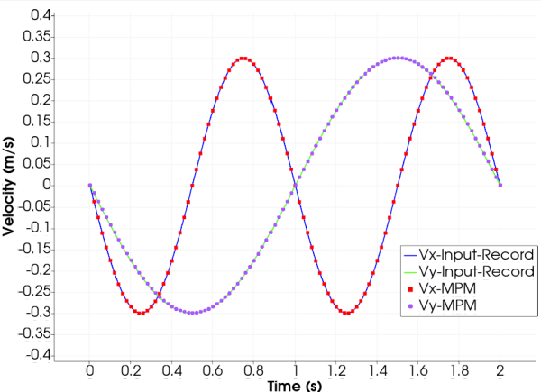
In order to validate the implementation of the dynamic boundary condition the velocity calculated from the input function used to created the base acceleration, \( \dot{u} = A sin ( 2 \pi f t + \alpha ) \) is compared with the velocity of a particle located at the base of the MPM model. The next figure shows this comparison. The velocities obtained with MPM at the base of the models coincides with the velocities obtained from the input record.